A brief introduction to wall functions in CFD

1.6K

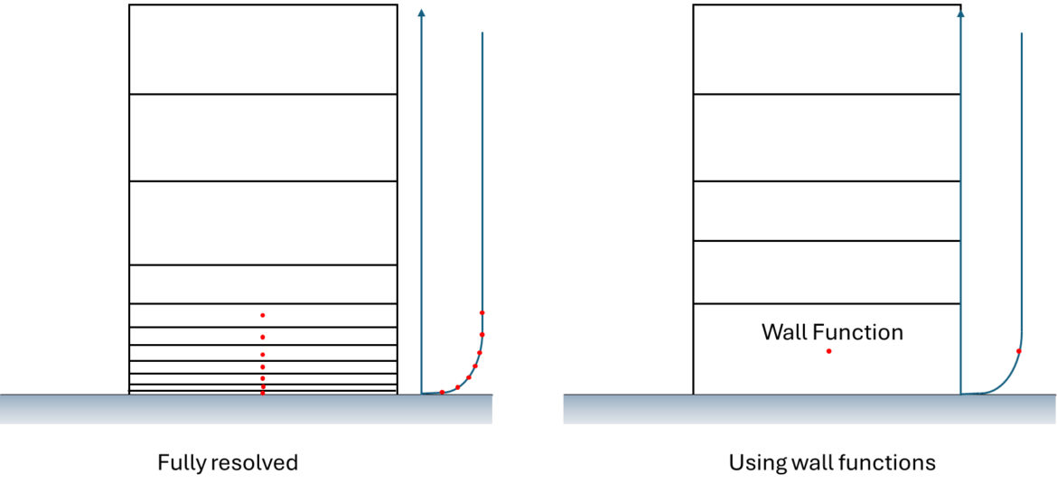
If you are a CFD engineer or scientist, wall functions are your best choice most of the time for your turbulent flow simulations since they can provide reliably accurate results within much less time than fully solving the turbulent boundary layer. This is especially true for unsteady simulations since you need many time steps to reach a steady-state or quasi-steady solution. So, what are the wall functions exactly? Before we talk about wall functions, we need to understand the law of the wall!

What is the law of the wall?

Turbulent boundary layer can be generally divided into three main regions:

1. Viscous sublayer

2. Buffer layer 

3. Log layer.

There are several experimental and computational databases available to support this approach as shown in the following figure (x axis is the distance from the wall and y axis is the non-dimensional near wall velocity.

You may easily notice that inside the viscous layer, the near wall velocity U+ can be expressed as:

where U+ is the near wall velocity and y+ is the non-dimensional wall distance (I assume you know these because you are reading my blog. If you are not sure, please refer to textbooks like Ferziger and Peric). Inside the buffer layer U+ becomes as follows:

Where k (it’s kappa) is the von Karman constant (around 0.41) and C is a constant (around 5.1). And this combined expression is called the law of the wall or the log-law. As you may notice, we have Spalding and Reichardt laws in our figure which are modified laws of the wall in order to satisfy the non-slip boundary condition at the wall. For your interest, the baseline (and the most popular) law of the wall does not satisfy the non-slip boundary conditions at the wall.

So, what is the deal with U+ and why wall functions are important? 

Basically, we need to model the near wall flow features properly by realizing the law of the wall inside our CFD analysis when using Reynolds Average Navier-Stokes (RANS) turbulence models. There are two ways. The first is to directly resolve the whole phenomena by putting cells (or) grid points inside the viscous sublayer. In other words, refining the mesh to obtain y+ values less than 1. This is not very attractive for most engineering problems where the boundary layer is so thin that you would need more than half of your cell count just inside the boundary layer mesh.

The second and more efficient approach is to use wall functions. Wall functions are empirical relationships used to approximate the behavior of the law of the wall by computing the wall distance to the nearest cell center and computing y+. When you have y+, you will have U+ from the law of the wall. This will save you from having to create a very fine boundary layer mesh and consequently tons of computational hours while providing you with sufficiently accurate results for most of your problems. (If you are interested in CFD meshing, you may be interested in our article about snappyHexMesh here.)

The limitations of wall functions

There is no free-lunch. Even in CFD. Wall functions come with limitations, like any other good things in our universe. The first limitation is accuracy. Although wall functions generally provide sufficiently accurate results for most engineering problems, if accuracy is of utmost importance, you may want to fully resolve the boundary layer with a very fine mesh.

The second limitation is the grid dependence. You need to adjust your wall functions or decide whether you should use wall functions or not based on the wall distance y+ of your mesh. For example, if your mesh is very fine (y+ < 1) and you use wall functions, your simulation will give you very strange results!

Summary

Wall functions are an essential tool in CFD for modeling turbulent flows near solid boundaries. By using empirical relationships to approximate the near-wall region, they provide a balance between accuracy and computational efficiency. Understanding how to apply wall functions correctly is crucial for achieving reliable simulation results in practical engineering applications.